Importing the Weather Data

Learning Objectives

Import a weather file to use real outdoor temperature data

Weather Data

So far we have had a constant outdoor temperature, but in reality this varies a lot. One way of accessing the weather data is through an epw file. For this exercise we will use the epw weather file for Zurich which can be downloaded from here

For a list of other locations, see the energy plus weather file website https://energyplus.net/weather

Importing the data

We will import the whole weather file as a pandas data frame for simplicity

Have a look at the 10 minute guide to pandas if you are not familiar with it

#Import Libraries
import numpy as np
import pandas as pd
# Set EPW Labels and import epw file
epw_labels = ['year', 'month', 'day', 'hour', 'minute', 'datasource', 'drybulb_C', 'dewpoint_C', 'relhum_percent',
                      'atmos_Pa', 'exthorrad_Whm2', 'extdirrad_Whm2', 'horirsky_Whm2', 'glohorrad_Whm2',
                      'dirnorrad_Whm2', 'difhorrad_Whm2', 'glohorillum_lux', 'dirnorillum_lux', 'difhorillum_lux',
                      'zenlum_lux', 'winddir_deg', 'windspd_ms', 'totskycvr_tenths', 'opaqskycvr_tenths', 'visibility_km',
                      'ceiling_hgt_m', 'presweathobs', 'presweathcodes', 'precip_wtr_mm', 'aerosol_opt_thousandths',
                      'snowdepth_cm', 'days_last_snow', 'Albedo', 'liq_precip_depth_mm', 'liq_precip_rate_Hour']

# Import EPW file
weather_data = pd.read_csv(epwfile_path, skiprows=8, header=None, names=epw_labels).drop('datasource', axis=1)

Reading the Imported Pandas DataFrame

The outdoor temperature for a particular hour of the year can now be read as


weather_data['drybulb_C'][hour]

where hour is an interger between 0 and 8759 which represents the 8760 hours of the year.

In the same way we can read all the other parameters of this weather file

New Simulation

For this new simulation we will use a time step of 1 hour for simplicity

# Import Libraries for Plotting
import numpy as np
import pandas as pd ## NEW!!!
import matplotlib.pyplot as plt

# Set EPW Labels and import epw file
epw_labels = ['year', 'month', 'day', 'hour', 'minute', 'datasource', 'drybulb_C', 'dewpoint_C', 'relhum_percent',
                      'atmos_Pa', 'exthorrad_Whm2', 'extdirrad_Whm2', 'horirsky_Whm2', 'glohorrad_Whm2',
                      'dirnorrad_Whm2', 'difhorrad_Whm2', 'glohorillum_lux', 'dirnorillum_lux', 'difhorillum_lux',
                      'zenlum_lux', 'winddir_deg', 'windspd_ms', 'totskycvr_tenths', 'opaqskycvr_tenths', 'visibility_km',
                      'ceiling_hgt_m', 'presweathobs', 'presweathcodes', 'precip_wtr_mm', 'aerosol_opt_thousandths',
                      'snowdepth_cm', 'days_last_snow', 'Albedo', 'liq_precip_depth_mm', 'liq_precip_rate_Hour']

# Import EPW file
weather_data = pd.read_csv(epwfile_path, skiprows=8, header=None, names=epw_labels).drop('datasource', axis=1)


# Set Boundary Conditions
T_in = 20.0 # Starting internal temperature [C]

# Initialise a list for collecting teperature data for plotting
list_T_in = []
list_T_out = []

#Set Building Parameters
C_m = 500.0 #[Wh/K]
R_total = 0.057 # [K/W]



# Set Integration Parameters
dt = 1.0 # delta time [hours] ##NEW!!!
simulation_time = 168.0 # length of simulation[hours]

for k in range (int(simulation_time / dt)):
 T_out =  weather_data['drybulb_C'][k]

 T_in = T_in + ((T_out - T_in)/(C_m * R_total)) * dt

 list_T_in.append(T_in) 
 list_T_out.append(T_out)

#Plotting

plt.plot(np.arange(0.0, simulation_time, dt),list_T_in, label = 'Indoor Temerature') 
plt.plot(np.arange(0.0, simulation_time, dt), list_T_out,label = 'Outdoor Temerature')
plt.xlabel('Time (Hours)')
plt.ylabel('Temperature (C)')
plt.legend()
plt.show()

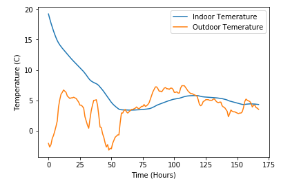
Interpretting the Results

What you are seeing is the initial decay of the indoor temperature to the outdoor temperature over the first week of January. After approximately 60 hours the indoor temperatures overlap. The lag between changes in the indoor and outdoor temperatures is due to the capacitance of the room

Tasks

Try run the same simulation for the whole year, so for 8759 hours
Try run the same simulation for a week in summer
What happens when you increase / decrease the thermal capacitance?

Importing Weather Data